Where magnetic fields come from: magnets, Earth and every electric current. Round a long straight wire the field B circles the wire and weakens with distance as B=μ0I/(2πr).
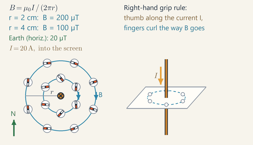
Compasses around a wire, seen from above: when a current flows, the needles swing into circles around the wire, and they turn round when the current is reversed.
A compass needle is a tiny magnet: it points along the field, whose lines run out of a magnet's north pole and round into its south pole.
Earth is a giant magnet. The magnetic pole under the Arctic is really a south pole, so it pulls the north end of every compass.
An electric current makes a magnetic field: around a straight wire, compass needles turn to form a ring.
Reverse the current and the ring reverses. Right hand: thumb along the current, fingers curl the way the field goes.
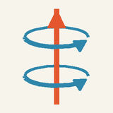
A coil carrying a current is an electromagnet you can switch off; an iron core inside makes it far stronger.
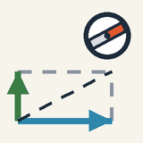
Hang a bar magnet from a thread and it settles with one end towards the north. That end is its north pole, the other its south pole. Two like poles push each other away; a north and a south pull together.
A compass needle is just a small magnet on a pivot. Wherever you place it, its north end shows the direction of the magnetic field at that spot. Move it around a magnet and you can trace the field lines: they leave the north pole, curve round and enter the south pole.
Earth is a giant magnet too, with a twist. Since unlike poles attract, the magnetic pole hidden under the Arctic must really be a south pole: that is why it pulls the north end of every compass.
In 1820 Hans Christian Ørsted found that a wire carrying a current also makes a magnetic field. The animation repeats his experiment, seen from above: small compasses sit around an upright wire. With no current they all point north. Switch on, and they swing into a ring around the wire; reverse the current and the ring turns the other way. To remember which way, grip the wire with your right hand, thumb along the current: your fingers curl the way the field goes.
Wind the wire into a coil and the rings add up inside it: you get an electromagnet that you can switch off. Soft iron inside makes it far stronger. Even a fridge magnet works this way, its electrons circling and spinning like tiny currents, all lined up.
Check yourself: a compass sits just north of an upright wire whose current flows upward. Where does its needle point? Answer: west, because seen from above, the field circles anticlockwise.
Intermediate
Key ideas
Long straight wire: B=μ0I/(2πr), with μ0=4π×10−7T⋅m/A; doubling r halves B.
Right-hand grip rule: thumb along the current, fingers curl the way the field lines go.
20 A gives 200 µT at 2 cm and 100 µT at 4 cm, ten and five times Earth's horizontal 20 µT.
A compass shows the total field, the wire's plus Earth's, so far from the wire it leans back towards north.
Solenoid: B=μ0nI inside, with n=N/L turns per metre; an iron core makes it far stronger.
What a magnetic field is, and how strong
A wire with no magnet in it turns a compass needle once a current flows through it. A magnetic field is what turns a compass needle near a magnet or a current. It has a direction, the way a compass's north end settles, and a size, the magnetic flux density B, measured in tesla (T): in 1 T, a wire carrying 1 A across the field is pushed with 1 N on every metre.
A tesla is a lot: a fridge magnet gives a few millitesla and an MRI scanner 1.5–3 T, while Earth's field is only 25–65 µT. A compass lying flat feels only its horizontal part, about 20 µT in mid-latitudes, the green value in the animation.
Field lines run the way a compass points, crowd where the field is strong and never cross; round a bar magnet they leave the north pole and curve into the south pole. Earth's magnetic pole under the Arctic attracts the north end of every compass, so it is a south pole.
The field of a long straight wire
In 1820 Hans Christian Ørsted saw a compass needle swing when he switched on a current in a nearby wire: electric currents make magnetic fields. The field lines of a long straight wire are circles centred on it, so the needle turns sideways, and iron filings on a card round the wire form rings. At a distance r from the wire B=2πrμ0I
where I is the current and μ0 is the magnetic constant, μ0=4π×10−7T⋅m/A Double I and B doubles; double r and B halves. A handy shortcut is μ0/(2π)=2×10−7T⋅m/A, so that B=2×10⁻⁷I/r with I in amperes and r in metres.
Which way it goes: reading the diagram
The direction comes from the right-hand grip rule: grip the wire with your right hand, thumb along the current, and your fingers curl the way the field lines go. The rule uses the conventional current I; in a metal the electrons drift the other way.
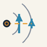
The animation looks down on the card, so the wire is seen end-on: a dot (•) means current out of the screen, like an arrow's tip, and a cross (×) current into it, like its feathers. With I=20A out of the screen your thumb points at you and the field circles anticlockwise: the blue B arrows on the east side point north. When the current reverses, the arrows flip and every needle swings round; the B readouts, which give only the size of the field, stay the same.
The inner needles, in the stronger field, swing faster than the outer ones, because the twist a field gives a magnet grows with B.
Loops and solenoids
Bend the wire into a circular loop of radius R and every part of it sends its field through the middle in the same direction. At the centre B=2Rμ0I(centre of a loop) which is π times what a straight wire gives at the distance R; a flat coil of N turns gives N times as much.
Stack many turns along a tube and you have a solenoid. Inside a long solenoid the fields of the turns add up to a nearly uniform field along the axis, while outside they almost cancel: B=μ0nI,n=LN Here n is the number of turns per metre, N turns over a length L; the radius does not matter if the coil is long compared with its width. The ends act like a bar magnet's poles: curl your right fingers along the current in the turns and your thumb points to the north end. With a soft-iron core inside, the coil becomes an electromagnet.
Worked example: the compasses in the animation
The wire carries I=20A, and the compasses sit 2 cm and 4 cm from it. With the distances in metres: B1=0.022×10−7⋅20=2.0×10⁻⁴T=200μT B2=0.042×10−7⋅20=1.0×10⁻⁴T=100μT
These are the two blue readouts, ten and five times Earth's horizontal 20 µT. A compass, though, shows the total field, the wire's plus Earth's. For the inner compass due north of the wire, the wire's field points west and Earth's north, so the needle turns from the circle towards north by an angle whose tangent is 20/200: about 5.7°. At 4 cm the ratio is 20/100, and the outer needles lean towards north by up to about 11°.
Where would the wire's field match Earth's BE=20μT? r=2πBEμ0I=20×10−62×10−7⋅20=0.20m With the current out of the screen, the field 20 cm due west of the wire points south and cancels Earth's: a compass there has no preferred direction. Due north, the two fields add at right angles to about 28 µT, and the needle points north-west. Reversing the current moves the cancelling point to the east.
Worked example: winding an electromagnet
You want 10 mT inside a coil 25 cm long, with wire rated for 2 A. Solve B=μ0nI for the turns per metre: n=μ0IB=4π×10−7⋅20.010≈4.0×10³m−1 That is about 4000 turns per metre, or N=nL=4000⋅0.25=1000 turns, and B=4π×10−7⋅4000⋅2≈1.0×10⁻²T, about 500 times Earth's horizontal field.
On a tube of radius 2 cm the coil uses 1000⋅2π⋅0.02≈126m of wire. In copper of cross-section 0.5 mm² its resistance is ρℓ/A=1.7×10−8⋅126/(0.5×10−6)≈4.3Ω, so 2 A needs about 8.5 V and turns 17 W into heat.
A soft-iron core lines up its atomic magnets with the coil's field and multiplies it many times: to a few tenths of a tesla in a straight rod, and to nearly 2 T, where iron saturates, in a closed iron path such as a lifting magnet's.
Common mistakes
Field lines of a wire are circles, not spokes: a compass 2 cm north of a wire carrying 20 A upwards points almost west.
The field of a long wire falls as 1/r, not 1/r2: 100 µT at 4 cm becomes 50 µT at 8 cm, not 25 µT.
Distances go in metres: r=2 instead of 0.02 gives 2 µT instead of 200 µT. Likewise n counts turns per metre: 1000 turns on 25 cm is n=4000m−1, not 1000.
A compass shows the total field, not the wire's alone: 20 cm from the animation's wire the two are equal, and the needles stop following the circles.
A mains cable carrying 10 A leaves a compass alone: its two conductors carry opposite currents a few millimetres apart, leaving about 1 µT at 10 cm instead of 20 µT for one alone, and the current reverses 100 times a second.
Where you meet it
Electromagnets lift scrap steel, hold fire doors open and switch relays. A loudspeaker drives its cone with a coil in a magnet's field, and an MRI scanner is a large solenoid: 1.5 T needs nI≈1.2×10⁶A/m, say 2000 turns per metre carrying 600 A, so its coil is cooled until it superconducts.
Next, Magnetic Force on Moving Charges shows what a field does to a current, Electromagnetic Induction how a changing field drives one, and Motors, Generators and Transformers uses both.
Advanced
Key ideas
Ampère's law ∮B⋅dl=μ0Ienc on a circle round the wire gives B⋅2πr=μ0I, so Br is constant.
Inside a wire of radius a with uniform current, B=μ0Ir/(2πa2): zero on the axis, largest at the surface.
Biot–Savart, dB=(μ0/4π)Idl×r^/r2, handles any shape: B=μ0I/(2R) at the centre of a loop.
A rectangle half inside a long solenoid gives a uniform B=μ0nI inside and almost no field outside.
∇⋅B=0: field lines always close, even through a magnet, and no magnetic monopole has ever been found.
Two local laws for steady currents
Every steady magnetic field obeys two rules. Everything else in the lesson, from the straight wire to the coaxial cable, follows from them.
For currents that do not change in time, the magnetic field B satisfies ∇⋅B=0,∇×B=μ0J Here J is the current density, the current per unit area of cross-section (A/m²), and μ0=4π×10−7T⋅m/A is the magnetic constant. The divergence ∇⋅B measures how much field flows out of a tiny volume; the curl ∇×B measures how much it circulates round a tiny loop.
The first law says that no net flux of B leaves any closed surface. Field lines therefore never start or end, because there are no magnetic charges. The lines of E in Electric Field and Potential, by contrast, start and end on charges.
The second law says that B circulates round currents, and only round currents. Where J=0, the field has no curl at all.
Ampère's law: circulation counts current
The curl law holds point by point. To use it on a real wire we need a form that adds up the circulation round a whole loop. Integrate the curl law over any surface bounded by a closed loop C: Stokes' theorem turns the left side into a line integral round C, and the right side becomes μ0 times the current Ienc that crosses the surface. The result is Ampère's law: ∮B⋅dl=μ0Ienc
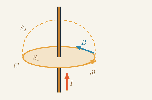
Figure 1. A closed loop C round a wire carrying I upwards, and two surfaces it bounds: the flat disc S1 and the dashed dome S2. Notice that the wire pierces both, and that the steps dl and the field B circle the way the right-hand fingers curl.Legend
I
Current in the wire, upwards. It crosses S1 and S2 alike, so it is the Ienc of Ampère's law.
A
C
Closed loop round which B is added up.
S1
Flat disc bounded by C.
S2
Dome bounded by the same loop C; the wire pierces it too.
dl
Short step along C, in the sense the right-hand fingers curl when the thumb points along I.
m
B
Magnetic field on C; it circles the wire in the same sense as the steps.
T
In Figure 1 the loop C is cut into small steps dl. At each step, take the part of B along the step and multiply it by the step's length. The left side of the law is the sum of these products all the way round C.
The direction of travel fixes the sign. Point your right thumb along a current: if your fingers curl the way the steps go, that current counts as positive. Here the wire carries I upwards, so the steps run anticlockwise as seen from above. The field B circles the wire the same way, so every product is positive.
Ienc is the current crossing a surface bounded by C. The obvious choice is the flat disc S1. But the dashed dome S2 has the same edge C, and the law does not say which surface to use, so both must give the same answer. In Figure 1 they do: the wire pierces S1 and S2 alike, so each is crossed by I.
This agreement is not automatic. The divergence of any curl is zero, so taking the divergence of the curl law gives ∇⋅J=0: charge never piles up, current flows round closed circuits, and every surface spanning C carries the same current. A charging capacitor breaks this. A dome that passes between its plates is crossed by no current, while the flat disc is crossed by the wire. That is the first sign that changing fields need an extra term, met at the end of this lesson.
The straight wire, outside and inside
Ampère's law gives B in one line, but only when symmetry tells us in advance that the field is the same all round the loop. The long straight wire is the cleanest case, and it shows how the symmetry argument goes.
A long straight wire looks the same after you slide along it or turn about it. So each part of B can depend only on the distance r from the wire. Split B into three parts: radial (pointing away from the wire), along the wire, and circling it.
The radial part is zero. Take a closed cylinder of radius r round the wire. Its two flat ends cancel, because the field along the wire is the same at both, entering one as it leaves the other. A radial part would then leave the curved side everywhere and give a net flux, which ∇⋅B=0 forbids.
The part along the wire is zero outside it. Take a rectangle in a plane through the wire, with both long sides outside the wire and on the same side of it. It encloses no current. Its short sides are radial, where the field has no part, so the two long sides must cancel: the field along the wire is the same at every distance. Far away it must vanish, so it vanishes everywhere outside.
What remains circles the wire, with a size B that depends only on r. Round a circle of radius r centred on the wire, B always points along the step, so the left side of Ampère's law is B⋅2πr. Setting this equal to μ0I gives B=2πrμ0I
Inside a wire of radius a that carries its current uniformly, a circle of radius r<a encloses only part of the current. That part is the ratio of the areas, πr2/(πa2)=r2/a2. So B⋅2πr=μ0Ir2/a2, and B=2πa2μ0Ir The field is zero on the axis and rises linearly to μ0I/(2πa) at the surface: 4.0 mT for 20 A in a wire of radius 1 mm. Outside, it falls as 1/r. Figure 4, further down, draws Ampère circles in both regions.
The solenoid: a uniform field inside
A solenoid is a long coil of wire, the standard way to make a uniform field. Ampère's law shows why with a single rectangle that lies half inside the coil and half outside.
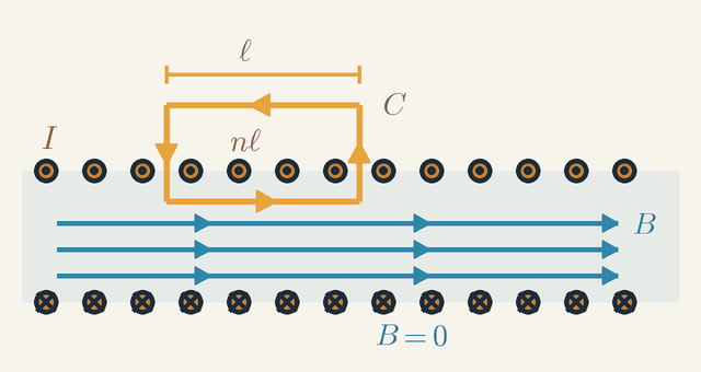
Figure 2. A long solenoid cut along its axis: dots are current out of the page, crosses current into it. Notice the rectangle C: its inner side, of length ℓ, runs along B; its outer side lies where B=0; nℓ turns pass through it.Legend
C
Rectangular loop for Ampère's law, run anticlockwise.
ℓ
Length of the two sides of C parallel to the axis.
m
I
Current in each turn: out of the page at the top, into it at the bottom.
A
B
Field inside the solenoid, along the axis; it is zero outside.
T
nℓ
Number of turns passing through C; n is the number of turns per metre.
Figure 2 cuts a long solenoid along its axis. In the top row the current comes out of the page (dots); in the bottom row it goes into the page (crosses). Curl the fingers of your right hand along the current in the turns, and your thumb gives the field inside: along the axis, to the right, as the arrows B show.
Outside the coil the field is zero. A rectangle lying wholly outside encloses no current, so its two long sides, parallel to the axis, must cancel: the field along the axis is the same at every distance outside. Far from the coil it must die away, so it is zero everywhere outside. That is the B=0 below the coil.
Now follow the rectangle C of Figure 2 round. Its inner side, of length ℓ, runs along the axis inside the coil, in the direction of B, and contributes Bℓ. Its outer side lies where B=0 and contributes nothing. Its two short sides cross the axial field at right angles inside the coil and lie in zero field outside, so they add nothing either. The left side of Ampère's law is just Bℓ.
On the right side, C is threaded by nℓ turns, where n is the number of turns per metre, and each carries I. So Ienc=nℓI, and Bℓ=μ0nℓI gives B=μ0nI Nothing in this depends on how far the inner side is from the axis, so the field is the same everywhere inside: uniform. It depends on the turns per metre and the current, not on the radius of the coil.
The B(r) graph and circles of equal flux
At the Advanced level the animation plots the field of the 20 A wire, B against r from 1 to 6 cm. This section reads that graph and shows why Ampère's law fixes its shape.
The curve is the hyperbola Br=μ0I/(2π)=4.0×10−6T⋅m, or 400 µT·cm. It passes through 400 µT at 1 cm, the marked 200 µT at 2 cm, 100 µT at 4 cm and 67 µT at 6 cm. On log–log axes it would be a straight line of slope −1, against −2 for a point charge and −3 for a distant magnet.
The constant product Br is exactly what Ampère's law demands. Take a loop that encloses no current: out along a radius from 2 to 4 cm, round the 4 cm circle through an angle Δφ, in along another radius, and back round the 2 cm circle. On the radial parts B is at right angles to the path, so they contribute nothing. The outer arc runs with the field and gives 100μT⋅4cm⋅Δφ; the inner arc runs against it and gives −200μT⋅2cm⋅Δφ. The two cancel, as they must with no current inside. A field falling faster or slower than 1/r would fail this test.
The flux through a strip in a plane through the wire, one metre long and reaching from r1 to r2, is the sum of Bdr across it: Φ=2πμ0Ilnr1r2 It depends only on the ratio r2/r1, so every doubling of r adds the same 2.8×10⁻⁶T⋅m2. Field lines drawn at equal steps of flux are therefore circles of radius 1, 2, 4 and 8 cm, spreading out as the field weakens; the two dashed circles of the animation are neighbours in such a set.
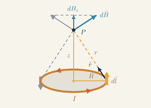
The Biot–Savart law: a loop seen from its axis
Ampère's law gives B only when symmetry keeps the field constant along some loop. Round a single circular coil no such loop exists, so we need a law that works for a circuit of any shape. The Biot–Savart law builds the field from short pieces of current: dB=4πμ0r2Idl×r^ Here dl is a short element of wire pointing along the current, r is its distance from the field point and r^ is the unit vector from the element towards that point. Each element adds a contribution that falls as 1/r2 and points at right angles to both the current and the line of sight.
Figure 3. A circular loop of radius R and a point P on its axis at height z. The element dl gives dB at right angles to the line r. Notice that the grey element opposite cancels the sideways part, leaving dBz=dBR/r. Not to scale.Legend
I
Current in the loop, anticlockwise as seen from above.
A
R
Radius of the loop.
m
z
Height of P above the centre of the loop, along the axis.
m
P
Point on the axis where the field is found.
r
Distance from the element dl to P, equal to R2+z2.
m
r^
Unit vector from the element towards P.
dl
Short element of the loop, on the right where the current runs into the page; drawn as up in this tilted view.
m
dB
Field of that element at P, at right angles to dl and to r^.
T
dBz
Axial part of dB; the axial parts of all elements point up and add.
T
Figure 3 applies the law to a circular loop of radius R carrying I, at a point P on its axis a height z above the centre. Look first at the element dl on the right-hand side of the ring. There the current runs into the page; in this tilted view, into the page is drawn as up.
Two facts make this element easy. Its distance from P is r=R2+z2, by Pythagoras on the triangle with sides R and z. And dl, which runs along the ring, is at right angles to the line r, so the cross product has its full size: dB=μ0Idl/(4πr2). Its direction is at right angles to both dl and r^: up and away from the axis, as the arrow dB shows.
Now look at the grey element on the opposite side of the ring. Its current runs the other way, so its field is the mirror image: up and away from the axis on its own side. The sideways parts of the two cancel. Pairing every element with its opposite, all the sideways parts cancel, and only the axial parts dBz survive, all pointing up.
How big is dBz? The arrow dB is at right angles to the line r, so the small triangle formed by dB and dBz is similar to the large triangle with sides R, z and r. Hence dBz=dBR/r.
Every element is at the same distance r and gives the same ratio R/r, and the element lengths add up to the circumference 2πR. The sum is therefore just a product: B=4πr2μ0I⋅rR⋅2πR=2(R2+z2)3/2μ0IR2
Two limits check the result. At the centre, z=0, so r=R and every element is side-on, and B=μ0I⋅2πR/(4πR2)=μ0I/(2R). For 20 A in a loop of radius 2 cm that is 628 µT, π times the 200 µT of a straight wire at the same 2 cm.
Far along the axis, for z≫R, the bracket becomes z3 and B≈μ0IR2/(2z3): the field falls as 1/z3. At 20 cm the same loop gives only 0.62 µT, where a straight wire still gives 20 µT. A small loop is a magnetic dipole, with the same far field as a bar magnet. Every real circuit, return wires included, is a closed loop, so far enough away its field also falls as the cube of the distance.
Finite wires and short solenoids
The same sum handles straight pieces of wire and coils of finite length, and shows how good the ideal formulas are.
A straight segment of length ℓ, seen from a point at perpendicular distance r opposite its midpoint, gives B=2πrμ0I⋅(ℓ/2)2+r2ℓ/2 The first factor is the infinite-wire value; the second, always less than 1, is the correction for the missing ends. For a 1 m wire seen from 4 cm it is 0.9968, so the field falls only 0.3 % short.
For a solenoid six radii long, like the animation's, adding up the fields of its turns gives 95 % of μ0nI at the centre and 49 % at the ends, where the computed field lines fan out. The ideal B=μ0nI is the limit of a very long coil.
Worked problem: a coaxial return path
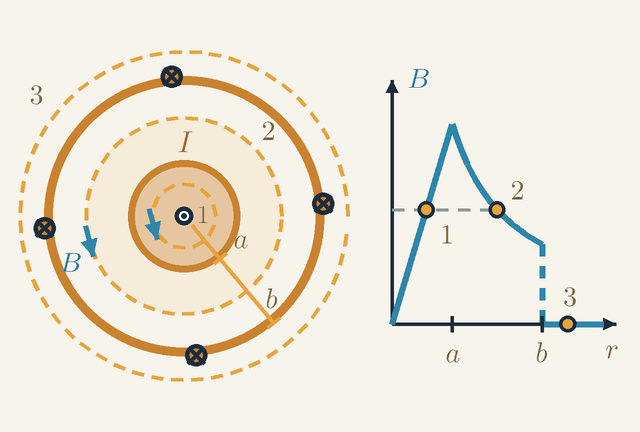
A coaxial cable sends a current out along a central rod and brings it back along a tube round it. It is a good test of Ampère's law, because the enclosed current changes from one circle to the next.
Let the animation's 20 A flow out of the screen along a copper rod of radius a=1cm and back into it through a thin tube of radius b=3cm round the rod. What do the compasses at 2 cm and 4 cm feel, and what is the field 0.5 cm from the axis?
Figure 4. A coaxial cable in cross-section (left) and B against r for the same circles (right). The rod carries I out of the page and the tube brings it back. Notice that circles 1 and 2 give the same B, and circle 3 gives none. Not to scale.Legend
I
Current in the rod, out of the page; the tube carries the same current back.
A
a
Radius of the rod.
m
b
Radius of the tube.
m
B
Size of the field on a circle of radius r round the axis.
T
r
Distance from the axis.
m
The left half of Figure 4 is the cross-section. The dot at the centre is the current I coming out of the page along the rod of radius a; the crosses are its return into the page along the tube of radius b. The dashed circles 1, 2 and 3 are Ampère loops at 0.5 cm, 2 cm and 4 cm. The drawing squeezes the radii to make room for the labels, so it is not to scale.
The cable looks the same after turning about its axis or sliding along it, just like the straight wire, so the field again circles the axis with a size that depends only on r. On each circle, Ampère's law gives B⋅2πr=μ0Ienc, or B=(μ0/2π)Ienc/r with μ0/(2π)=2×10−7T⋅m/A. The only work is finding Ienc.
Circle 1, inside the rod, encloses (0.5/1)2, a quarter, of the rod's area and so a quarter of its current. Circle 2 encloses all of the rod's current and none of the tube's. Circle 3 encloses both, and they cancel: Ienc(0.5cm)=20⋅(0.5/1)2=5A,B=0.0052×10−7⋅5=2.0×10−4T Ienc(2cm)=20A,B=200μT Ienc(4cm)=20−20=0,B=0
The right half of Figure 4 plots B against r for the whole cable. The field climbs in a straight line to a peak of 400 µT at r=a, follows the animation's 1/r hyperbola out to r=b, then drops to zero. Circles 1 and 2 sit at the same height: 200 µT inside the rod at 0.5 cm, and 200 µT outside it at 2 cm.
So the inner compasses, at 2 cm, notice nothing new: the tube's current lies outside their circle, and a uniform tube makes no field inside itself. The outer compasses, at 4 cm, feel only Earth's horizontal field of about 20 µT and point north as if the current were off.
If 5 A leaked to earth elsewhere, so that only 15 A came back through the tube, circle 3 would enclose 5 A. The outer compasses would then feel 2×10−7⋅5/0.04=25μT from the cable, more than Earth's field. A residual-current device uses exactly this: a ring round both conductors senses only their net current, the Ienc of Ampère's law, and cuts off the circuit when it is not zero.
One field seen from two frames
Magnetism is not a separate force. This section shows that the magnetic force of a wire is an electric force seen from another frame.
Let the wire be copper with a cross-section of 2.5 mm². Its mobile electrons carry about 3.4×10⁴C per metre of wire, balanced exactly by the positive ions, so the wire is neutral. To carry 20 A the electrons drift at only v≈0.59mm/s.
Now let a charge move alongside the wire, parallel to the electrons and at their speed v. In the lab it feels a magnetic force, because it moves through the field B. In its own frame it is at rest, and a magnetic field exerts no force on a charge at rest. The force cannot vanish by a change of viewpoint, so in that frame it must be electric.
It is. In the charge's frame the ions move, so their spacing is length-contracted and they are more crowded than in the lab. The electrons are now at rest, at their own natural spacing, which is wider than the contracted spacing seen in the lab, so they are less crowded. The wire is no longer neutral.
The two densities differ by a fraction v2/c2≈4×10−24: a net charge of less than one electron per metre of wire. Yet at 2 cm this tiny charge makes an electric field of 1.2×10⁻⁷V/m, the same as the vB of a charge moving at v through 200 µT. Electric and magnetic fields are two aspects of one field, mixed by a change of frame, with μ0ε0=1/c2 as the rate of exchange.
The right-hand rule is only a convention. B appears both in the field law and in the force qv×B, so a left-hand rule used in both would reverse B and change no prediction.
Permanent magnets obey the same equations. Their currents are inside atoms, above all the spins of electrons, lined up across whole domains in iron.
Limits of validity
These are the laws of steady currents. When currents change, Maxwell's term μ0ε0∂E/∂t joins μ0J in the curl law. It mends the charging capacitor of Figure 1, and it makes changes of the field spread at c=1/μ0ε0≈3.00×108m/s.
The static formulas still hold at distances much smaller than the wavelength. At 50 Hz the wavelength is 6000 km, so household wiring is magnetostatic; at 100 MHz it is 3 m, and a wire radiates.
The laws also assume empty space or air, whose permeability differs from μ0 by less than one part per million. The strongest steady laboratory fields are about 45 T, and magnetars, a kind of neutron star, reach about 1010T.
The magnetism of matter is quantum at heart. Classical physics predicts no magnetisation at all for charges in thermal equilibrium, and the alignment of spins in iron is a quantum effect.
Where this leads
Magnetic Force on Moving Charges adds the force qv×B, the attraction between parallel currents and the circular orbits of charged particles. Electromagnetic Induction shows that a changing B drives an electric field round a loop, the counterpart of Ampère's law, and Motors, Generators and Transformers uses coils and iron cores. With Maxwell's term, the two curl laws give the waves of Electromagnetic Waves, and the change of frame above is developed in Special Relativity.
Key formulas
Field of a long straight wire
B=2πrμ0I
The field lines of a straight current are circles round the wire, with the same field all along each circle. Ampère's law on such a circle gives B⋅2πr=μ0I, so the field is proportional to the current and falls as 1/r, more slowly than the 1/r2 of a point charge. Its direction follows the right-hand grip rule.
Symbols
B
magnetic field at distance r
T
μ0
magnetic constant
T⋅m/A
I
current in the wire
A
r
distance from the axis of the wire
m
When it holds: For a steady current in a straight wire much longer than r, outside the wire and with no iron nearby. Inside a wire of radius a with uniform current, B=μ0Ir/(2πa2) instead; a 1 m wire seen from 4 cm gives 0.3 % less than the formula.
Example: The animation's 20 A: B=2×10−7⋅20/0.02=200μT at 2 cm and 100 µT at 4 cm.
Magnetic constant
μ0=4π×10−7T⋅m/A
μ0 sets how strong a field a given current makes, in SI units. Until 2019 its value was exact by definition, because the ampere was defined through the force between two parallel wires; now the ampere is fixed through the charge of the electron and μ0 is measured, but it still equals 4π×10−7T⋅m/A to better than one part in a billion. Together with the electric constant it fixes the speed of light, μ0ε0=1/c2.
Symbols
μ0
magnetic constant (permeability of free space)
T⋅m/A
When it holds: The value for vacuum, and for air to within one part in a million. Inside a magnetic material such as iron the field is multiplied by the relative permeability of the material, which is not a constant.
Example:μ0/(2π)=2×10−7T⋅m/A, so for the animation's 20 A the product Br is 4.0×10⁻⁶T⋅m at every distance.
Field inside a long solenoid
B=μ0nI,n=LN
Inside a long coil the fields of all the turns add up to a uniform field along the axis, while outside they nearly cancel. Ampère's law round a rectangle with one side inside gives B=μ0nI: only the turns per metre and the current matter, not the radius. Seen from outside, the end round which the current flows anticlockwise is the north pole.
Symbols
B
magnetic field inside the solenoid
T
μ0
magnetic constant
T⋅m/A
n
number of turns per metre
m−1
I
current in the winding
A
N
total number of turns
L
length of the solenoid
m
When it holds: For a solenoid much longer than its radius, well inside it and away from the ends, where the field drops to about half; without an iron core, which multiplies the field until the iron saturates near 2 T.
Example: 1000 turns on 25 cm carrying 2 A: n=4000m−1 and B=4π×10−7⋅4000⋅2≈10mT.
Field at the centre of a circular loop
B=2Rμ0I(centre of a loop)
Every element of the loop is at the same distance R from the centre and at right angles to the line joining them, so the Biot–Savart contributions all point the same way, along the axis, and add up to μ0I⋅2πR/(4πR2). That is π times the field of a straight wire at the same distance. A flat coil of N turns gives N times as much.
Symbols
B
magnetic field at the centre of the loop
T
μ0
magnetic constant
T⋅m/A
I
current in the loop
A
R
radius of the loop
m
When it holds: Only at the centre. On the axis, at a distance z, the field is μ0IR2/[2(R2+z2)3/2], which far away falls as 1/z3, like the field of a small magnet.
Example: 20 A in a loop of radius 2 cm: B=4π×10−7⋅20/0.04≈628μT, π times the 200 µT that the straight wire gives at 2 cm.
Ampère's law
∮B⋅dl=μ0Ienc
Go round any closed loop and add up the component of B along the path times each step: this total, the circulation, equals μ0 times the current threading the loop. Currents outside the loop change B on it but add nothing to the circulation. With your fingers along the loop, a current along your right thumb counts as positive. The law follows from ∇×B=μ0J by Stokes' theorem.
Symbols
B
magnetic field at each point of the loop
T
dl
short step along the loop
m
μ0
magnetic constant
T⋅m/A
Ienc
net current through the loop
A
When it holds: True for any loop when the currents are steady, but it gives the field only when symmetry keeps the field constant along the loop (wire, solenoid, coaxial cable, ring-shaped coil). When fields change, a term proportional to the rate of change of the electric flux through the loop must be added to the current.
Example: Round the animation's wire at 2 cm: 200μT⋅2π⋅0.02m≈2.5×10⁻⁵T⋅m, which is μ0 times 20 A.
Biot–Savart law
dB=4πμ0r2Idl×r^
Each short piece Idl of a circuit contributes a field that falls as the inverse square of the distance, as in Coulomb's law, but points at right angles to both the current and the line from the piece to the field point. Because of the cross product the contribution is largest side-on and zero straight ahead along the wire. Adding the pieces of the whole circuit gives its field, whatever its shape.
Symbols
dB
field contributed by one element
T
μ0
magnetic constant
T⋅m/A
I
current in the circuit
A
dl
short piece of wire, pointing along the current
m
r^
unit vector from the element to the field point
r
distance from the element to the field point
m
When it holds: For steady currents, summed round complete circuits. For rapidly changing currents the delay of the field, which travels at c, must be included.
Example: For a loop of radius R every piece is side-on at the distance R, and the sum is μ0I/(2R); for a long straight wire the sum is μ0I/(2πr).
Glossary
Magnetic field
The property of the space round magnets and currents that turns compass needles and pushes on moving charges. It has a direction, the way the north end of a compass points, and a size, the flux density B in tesla.
Magnetic field line
A line drawn so that a compass placed on it points along it. Field lines crowd together where the field is strong, never cross, and close on themselves: round a straight wire they are circles.
Magnetic pole
An end of a magnet where field lines leave (north pole) or enter (south pole). Like poles repel and unlike poles attract; poles always come in pairs, and a magnet cut in two becomes two smaller magnets.
Earth's magnetic field
The field of the planet, made by currents in its liquid iron outer core: 25–65 µT at the surface. Its horizontal part, about 20 µT in mid-latitudes, sets compasses north; the magnetic pole under the Arctic is a south pole.
Ørsted's experiment
The discovery, in 1820, that a compass needle beside a wire turns when a current flows: the first link found between electricity and magnetism. The needle turns across the wire, not towards it.
Right-hand grip rule
Grip the wire with your right hand, thumb along the conventional current: your fingers curl the way the field lines go. For a coil, curl your fingers along the current in the turns and your thumb points to the north end.
Solenoid
A long coil of wire wound on a tube. Inside, its field is nearly uniform, B=μ0nI, whatever the radius; outside, the field is weak and has the pattern of a bar magnet's.
Electromagnet
A coil with a soft-iron core. The coil's field lines up the iron's atomic magnets, which multiply the field many times, and switching off the current lets the load go.
Magnetic domain
A region of a ferromagnet such as iron in which the atomic magnets all point the same way. An applied field grows the domains aligned with it; once all are aligned, near 2 T, the iron is saturated.
Ampère's law
The circulation of B round any closed loop equals μ0 times the current through the loop. With enough symmetry it gives the field of a wire, B⋅2πr=μ0I, or of a solenoid in one line.
Biot–Savart law
The field of a short piece of current: at right angles to the current and to the line of sight, and falling as 1/r2. Adding the pieces gives the field of any circuit, such as μ0I/(2R) at the centre of a loop.
Magnetic monopole
A hypothetical isolated north or south pole, a magnetic charge. None has ever been found, which is what ∇⋅B=0 expresses: field lines have no beginning and no end.
Quantities
B
Magnetic field (flux density)
T
The strength of the magnetic field at a point. Earth's horizontal field is about 20 µT; the animation's wire gives 200 µT at 2 cm.
μ0
Magnetic constant
T⋅m/A
Sets how strong a field a current makes in SI units: 4π×10−7T⋅m/A, so that μ0/(2π)=2×10−7T⋅m/A.
I
Current
A
The charge passing per second. Its conventional direction, the way positive charge would flow, sets the direction of the field.
r
Distance from the wire
m
Measured at right angles from the axis of the wire; the field falls as 1/r. In the Biot–Savart law r is instead the distance from a current element to the field point, along the unit vector r^.
R
Radius of the loop
m
The radius of a circular current loop, which is also the distance of every part of it from the centre.
N
Number of turns
How many times the wire is wound round a coil or solenoid.
L
Length of the solenoid
m
The length over which the turns are wound; the formula for B inside needs it to be much larger than the radius.
n
Turns per unit length
m−1
n=N/L: 1000 turns over 25 cm give n=4000m−1.
Ienc
Enclosed current
A
The net current through any surface bounded by an Ampère loop, counted positive along the right thumb when the fingers follow the loop.
dl
Line element
m
A short directed step along an Ampère loop, or a short piece of wire pointing along the current in the Biot–Savart law.
Quiz
Beginner A compass sits next to a wire. What happens to its needle when a current is switched on in the wire?
Nothing: only magnets can move a compass needle
It turns, because the current makes a magnetic field around the wire
It spins round and round for as long as the current flows
It swings round to point straight at the wire
Show answer
Answer: B. It turns, because the current makes a magnetic field around the wire
An electric current produces a magnetic field, as Ørsted discovered in 1820. The needle turns to line up with that field, along a circle around the wire, and then stays still.
Beginner A straight wire carrying a current passes upright through a card, and iron filings are sprinkled on the card. What pattern do they form?
Straight lines pointing away from the wire
Parallel lines running north–south
Circles centred on the wire
No pattern, because a wire is not a magnet
Show answer
Answer: C. Circles centred on the wire
The field lines of a straight current are circles around the wire, and the filings line up along them.
Beginner Two bar magnets are pushed together with their north poles facing each other. What do you feel?
They push each other apart
They pull together
Nothing, unless one of them is made of iron
They pull together at first, then push apart
Show answer
Answer: A. They push each other apart
Like poles repel and unlike poles attract, so two north poles push each other apart.
Intermediate A long straight wire carries 10 A. What is the magnetic field 5 cm from it? (μ₀ = 4π × 10⁻⁷ T·m/A)
2.0 × 10⁻⁵ T
4.0 × 10⁻⁷ T
1.3 × 10⁻⁴ T
4.0 × 10⁻⁵ T
Show answer
Answer: D. 4.0 × 10⁻⁵ T
B = μ₀·I/(2π·r) = 2 × 10⁻⁷ × 10 / 0.05 = 4.0 × 10⁻⁵ T, or 40 µT. Leaving r in centimetres gives 4.0 × 10⁻⁷ T, and using the loop formula μ₀·I/(2r) by mistake gives 1.3 × 10⁻⁴ T.
Intermediate The field 3 cm from a long straight wire is 120 µT. What is it 6 cm from the wire?
240 µT
120 µT
60 µT
30 µT
Show answer
Answer: C. 60 µT
B is inversely proportional to r: doubling the distance halves the field, giving 60 µT. 30 µT would follow from an inverse-square law, which describes a point charge, not a long wire.
Intermediate A current flows straight up a vertical wire. Seen from above, which way do the magnetic field lines go round the wire?
Anticlockwise
Clockwise
Radially outwards, away from the wire
Straight up, along the current
Show answer
Answer: A. Anticlockwise
Right-hand grip rule: with your thumb pointing up along the current, your fingers curl anticlockwise when seen from above.
Advanced A long straight wire and a circular loop of radius R carry the same current I. How does the field at the centre of the loop compare with the wire's field at distance R?
They are equal
The loop's field is π times larger
The loop's field is twice as large
The loop's field is π times smaller
Show answer
Answer: B. The loop's field is π times larger
At the centre of the loop B = μ₀·I/(2R), while the wire gives μ₀·I/(2πR) at distance R: a ratio of π. Every element of the loop is at distance R and perpendicular to the line joining it to the centre, so all their contributions add up in the same direction.
Advanced A long straight wire of radius a carries a current I spread uniformly over its cross-section. How does B vary with the distance r from the axis inside the wire (r < a)?
B = 0 everywhere inside the wire
B = μ₀·I/(2π·r), as outside, so it is largest on the axis
B grows in proportion to r, reaching μ₀·I/(2π·a) at the surface
B is the same everywhere inside, equal to μ₀·I/(2π·a)
Show answer
Answer: C. B grows in proportion to r, reaching μ₀·I/(2π·a) at the surface
A circle of radius r < a encloses the current I·r²/a², so Ampère's law gives B·2πr = μ₀·I·r²/a² and B = μ₀·I·r/(2πa²): zero on the axis, rising linearly to the surface value.
 Physics Tutor