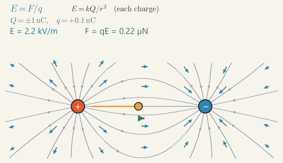
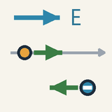
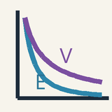
A charge Q fills the space around it with an electric field E, the force on each coulomb, and a potential V, the energy of each coulomb: a positive charge is pushed along E, from high V to low V.
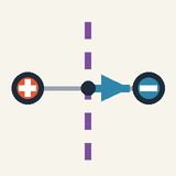
The field lines of a positive and a negative charge, with a small positive test charge released near the + charge. It accelerates along the central field line towards the − charge.
Like charges repel, opposite charges attract, even without touching; twice the distance gives a quarter of the force.
A charge fills the space around it with an electric field: the push a small + charge would feel there.
Field lines leave + charges and end on − charges; where they crowd together the push is strong.
Field strength is the force on each coulomb: in 100 N/C, half a coulomb feels 0.5×100=50N.
Voltage is like height on a hill: a + charge falls from high to low voltage and speeds up; 1 volt = 1 joule per coulomb.
Rub a balloon on your hair and it can lift the hair from a few centimetres away. Electric charges push and pull without touching, and the basic rule is short: like charges repel, opposite charges attract. The force also fades fast with distance: move two charges twice as far apart and it drops to a quarter.
Step 1: the field. Instead of tracking every charge, we say that each charge fills the space around it with an electric field. At any point, the field tells you which way, and how hard, a small positive "test" charge put there would be pushed. Around a + charge the field points outward; around a − charge it points inward.
Step 2: field lines. We draw the field as lines with arrows. They leave + charges and arrive at − charges. Where the lines crowd together the push is strong; where they spread out it is weak.
Step 3: how strong. Field strength is the force on each coulomb of charge, in newtons per coulomb (N/C). In a field of 100 N/C, a charge of half a coulomb feels 0.5×100=50N.
Step 4: voltage. Electric potential, measured in volts, works like height on a hill. A + charge "falls" from high voltage to low voltage and speeds up, the way a ball rolls downhill. A difference of one volt means each coulomb gains or loses one joule of energy.
In the animation, grey lines run from the + charge to the − charge and bunch up near each one. The small gold charge, released near the +, slides along the middle line, faster and faster.
Check yourself: in a field of 400 N/C, what force acts on a charge of 0.005 C? (Answer: 2 N.)
Intermediate
Key ideas
E=F/q: the force per coulomb on a small positive test charge, in N/C = V/m.
A point charge gives E=kQ/r2 (a vector) and V=kQ/r (a number that keeps the sign of Q).
Fields from several charges add as vectors; potentials add as plain numbers.
Moving q through ΔV changes its potential energy by ΔU=qΔV; 1eV=1.602×10⁻¹⁹J.
Zero potential does not mean zero field: midway between +Q and −Q, V=0 but E=0.
The field: force per unit charge
Charges push and pull each other across empty space, as Coulomb's Law describes. The field picture splits this into two steps: the source charges set up an electric field E everywhere around them, and a charge placed at a point feels the field right there.
To measure the field, place a small positive test charge q at the point, measure the force on it and divide: E=qF
Doubling q doubles the force, so the ratio belongs to the point, and the field is there even when nothing probes it. Its unit is the newton per coulomb, which equals the volt per metre. Turned around, F=qE: a positive charge is pushed along the field, a negative one against it. The animation's test charge, q=+0.1nC, is ten times smaller than the fixed sources, ±1nC.
Point charges and superposition
Dividing Coulomb's law by the test charge gives the field of a point charge Q at a distance r: E=r2kQ with k≈8.99×10⁹Nm2/C2. It points away from a positive Q and towards a negative one.
With several charges, each produces its own field as if the others were absent, and the total is their vector sum. On the perpendicular bisector of the animation's pair, the two fields are equally strong, one pointing away from the + charge and one towards the − charge. Their components across the axis cancel and those along it add, so the total runs parallel to the axis, towards the − side. The blue grid arrows show these sums, their lengths compressed to fit the strong field near the charges.
Potential: energy per unit charge
The potential describes the same field with one number per point instead of an arrow. Moving a charge against the electric force takes work, stored as electric potential energy U, just as lifting a stone stores gravitational potential energy. Per unit charge this becomes the electric potential V=U/q, measured in volts: 1V=1J/C.
When a charge q moves through a potential difference ΔV, its potential energy changes by ΔU=qΔV, and the field does work Wfield=−ΔU on it. A positive charge left to itself moves towards lower potential and speeds up, like a ball rolling downhill; an electron moves towards higher potential. An electron accelerated through 1 V gains one electron-volt, 1eV=1.602×10⁻¹⁹J.
With V=0 far away, a point charge has V=kQ/r: no square, and Q keeps its sign, so the potentials of several charges add as signed numbers. The field points towards lower potential, and its strength is how fast V falls per metre. Between parallel plates a distance d apart the field is uniform, E=ΔV/d. These are the working equations of this level:
E=qF
E=r2kQ
V=rkQ
ΔU=qΔV=−Wfield
E=dΔV(uniform field)
Worked example: the dipole in the animation
The source charges Q=±1nC are 180 mm apart, and the test charge q=+0.1nC starts at rest 20 mm from the + charge. At the midpoint each source is 0.090 m away and contributes r2kQ=0.09028.99×109⋅10−9≈1.11×10³V/m
Both contributions point towards the − charge, so E≈2.22kV/m and F=qE≈0.22μN. At the start the + charge, 0.020 m away, gives 22.5 kV/m and the − charge, 0.160 m away, adds 0.35 kV/m, so E≈22.8kV/m and F≈2.28μN, ten times more. These are the E and F readouts at the start and halfway, and the green force arrow is long at both ends of the trip and short in the middle.
At the start the potential is V=kQ/0.020−kQ/0.160=449.5−56.2≈393V; by symmetry it is −393V at the end and zero at the midpoint. Over this drop of 786.6 V the field does work W=10−10⋅786.6≈7.87×10⁻⁸J, the 78.7 nJ of kinetic energy on the expert layer's K readout. Half of it is gained by the midpoint, so the speed there is 1/2, about 71 %, of the final speed; starting from rest, the charge takes 2.45 s of its 4.0 s trip to get there.
Worked example: an electron between two plates
In an electron gun, electrons are pulled from a negative plate towards a positive one. Take plates 1.0 cm apart at 500 V, with an electron starting at rest; the field between them is uniform: E=dΔV=0.010500=5.0×10⁴V/m
The force, F=eE=1.602×10−19⋅5.0×104≈8.0×10⁻¹⁵N, points against the field, towards the positive plate; the electron's weight is about 1015 times smaller. Crossing the gap it gains 500 eV, or 8.0×10⁻¹⁷J, and with its mass m=9.11×10⁻³¹kg, 21mv2=eΔV gives v=m2eΔV=9.11×10−312⋅8.0×10−17≈1.33×10⁷m/s
That is about 4.4 % of the speed of light. The acceleration is constant, so the average speed is v/2 and the crossing takes t=2d/v≈1.5ns. Television tubes used about 25 kV, enough for nearly a third of the speed of light.
Reading the field map
A field line runs along E at every point, and its arrow shows where a positive charge would be pushed. Lines start on positive charges and end on negative ones, and in the animation as many reach the − charge as leave the + charge. They never cross, since the field has only one direction at each point, and where they crowd together, near the charges, the field is strong.
The dashed equipotentials of the expert layer cut every field line at right angles, since moving a charge along one takes no work; the straight one midway is V=0.
Common mistakes
Field lines are not paths: a charge released off the axis cuts across the curved lines, since its inertia keeps it from turning with them; the gold charge follows the central line only because it is straight.
The field is not the force: at the midpoint E=2.2kV/m for any test charge, but the force is 0.22 µN on 0.1 nC and 2.2 µN on 1 nC.
The potential falls as 1/r, the field as 1/r2: at 10 cm from 4 nC, forgetting the square gives 360 V/m instead of 3600 V/m.
Zero potential is not zero field: midway between the charges the potentials +99.9 and −99.9V cancel, while the fields add up to 2.22 kV/m.
A negative charge is pushed against the field and gains speed towards higher potential: the electron between the plates gains 500 eV going from 0 V to +500 V.
Where you meet it
Electric fields steer electrons in electron microscopes and ions in mass spectrometers, clean smoke out of chimney gases and place toner in laser printers. Dry air breaks down at about 3 MV/m, so a spark jumps a 1 mm gap at about 3 kV. Nerve cells hold about 70 mV across a membrane 7 nm thick, some 10 MV/m.
Next, Capacitors shows how the field between two plates stores energy, Electric Current and Resistance how a field drives charge through a wire, and DC Circuits and Ohm's Law how a voltage keeps charge moving round a circuit. The same mathematics, for masses that only attract, governs Gravitation and Orbits.
Advanced
Key ideas
Path independence, ∮E⋅dl=0, forbids perpetual motion from static charges and defines V with E=−∇V.
Energy conservation: K+qV is constant, so the speed gained depends only on the end points, not the route.
Field lines work because of the 1/r2 law (Gauss: ∇⋅E=ρ/ε0); they cross equipotentials at right angles.
In empty space ∇2V=0: no static field can trap a charge stably (Earnshaw).
With changing magnetic fields, E=−∇V−∂A/∂t and ∮E⋅dl=0: V alone no longer describes E.
Superposition solves electrostatics
One rule settles every static field. Everything later in the lesson is either a shortcut to it or a way of picturing its answer. When the source charges stay still, two facts are enough. Coulomb's law gives the field of a single charge: it points along the line through the charge, and its size falls as the inverse square of the distance. The principle of superposition says that the fields of several charges simply add as vectors, each charge acting as if the others were not there.
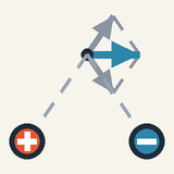
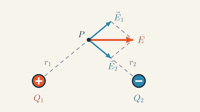
Figure 1. Superposition at a point P: E1 points away from the positive Q1, E2 towards the negative Q2. As P is equally far from both, their parts across the line of the charges cancel and the sum E, the diagonal of the dashed parallelogram, is parallel to the line of the charges.Legend
Q1
Positive source charge.
C
Q2
Negative source charge, here −Q1.
C
P
Point where the field is found.
r1
Distance from Q1 to P; equal to r2 here.
m
r2
Distance from Q2 to P; equal to r1 here.
m
E1
Field of Q1 alone at P, pointing away from Q1.
N/C
E2
Field of Q2 alone at P, pointing towards Q2.
N/C
E
Total field at P: the vector sum E1+E2.
N/C
Figure 1 adds two fields at one point P. The positive charge Q1 would push a positive test charge away, so its field E1 points from Q1 through P and beyond. The negative charge Q2 would pull the test charge in, so its field E2 points from P towards Q2. Each arrow has the size k∣Qi∣/ri2, where ri is the distance from charge Qi to P and k≈8.99×10⁹Nm2/C2 is the Coulomb constant.
Now look at where P sits: on the perpendicular bisector of the pair. So r1=r2, and the two arrows are equally long. Their parts at right angles to the line of the charges are equal and opposite, so they cancel. What survives is the sum E, the diagonal of the dashed parallelogram, and it runs parallel to the line from the positive charge to the negative one.
To write the same sum for any number of charges, put charge Qi at position ri and ask for the field at position r. The vector from the charge to the field point is r−ri, of length ri. Dividing it by ri3 leaves a unit vector divided by ri2: the inverse-square size, already pointing the right way. Adding over all the charges: E(r)=∑i∣r−ri∣3kQi(r−ri)
Charge spread out with density ρ, in coulombs per cubic metre, is cut into small pieces of charge ρd3s at points s, and the sum becomes an integral: E(r)=k∫∣r−s∣3ρ(s)(r−s)d3s
In principle nothing more is needed. The animation draws its field lines from exactly this two-term sum. The potential, field lines and Gauss's law below reach the same answer with less work, or show its shape at a glance.
The potential: work that ignores the route
Adding vectors at every point is laborious. A single number at each point, the potential, would be far easier to add up. Such a number exists only if the work the field does between two points is the same along every route. This section shows that it is.
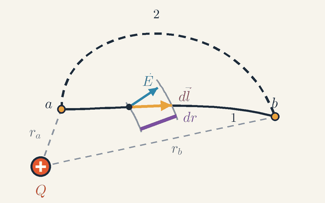
Figure 2. Two routes from a to b near a charge Q. A step dl changes the distance from Q by dr, the gap between the dashed arcs. Only dr counts in E⋅dl, so both routes give the same work.Legend
Q
Point charge that makes the field.
C
a
Start of both routes.
b
End of both routes.
ra
Distance from Q to a.
m
rb
Distance from Q to b.
m
dl
A small step along route 1: its length and direction.
m
dr
Change in the distance from Q over that step: the gap between the dashed arcs.
m
E
Field at the start of the step, pointing straight away from Q.
N/C
Figure 2 shows a point charge Q and two routes from point a to point b. Move a test charge along a route in small steps dl. On each step the field does work qE⋅dl on a charge q, so the work per unit charge from a to b is the line integral ∫abE⋅dl: the sum of E⋅dl over all the steps.
Look at the step drawn on route 1. The field E at its start points straight away from Q, so the dot product keeps only the part of the step along the radius. That part is dr, the gap between the two dashed arcs centred on Q: how much the step changes the distance from Q. Moving sideways, along an arc, costs no work at all. Hence E⋅dl=Edr=r2kQdr Adding the steps from distance ra out to distance rb: ∫abE⋅dl=∫rarbr2kQdr=kQ(ra1−rb1) The result depends on the end distances ra and rb and on nothing else. Route 2 is longer and swings far out above route 1, but between ra and rb it crosses the same set of circles around Q, so it collects exactly the same total.
Any static arrangement is a sum of point charges. Each term of that sum is independent of the route, so the whole field is too. Going out along one route and back along another therefore gives zero work round the closed loop: ∮E⋅dl=0 If this failed, a charge sent round the loop in the favourable direction would gain energy on every lap from charges that never change: a perpetual-motion machine.
Because the route does not matter, one number can be attached to each point: the electric potential V, in volts (joules per coulomb). Its change from a to b is defined as ΔV=Vb−Va=−∫abE⋅dl The minus sign makes V fall in the direction the field points. A positive charge pushed along by the field then loses potential energy qV and gains the same amount of kinetic energy. Choosing V=0 infinitely far away, and writing s for the distance from Q inside the integral, a point charge gives V(r)=−∫∞rs2kQds=rkQ
Read the other way round, the field is minus the gradient of the potential. It points the way V falls fastest, and its size is how many volts V falls per metre in that direction. Energy conservation for a charge q with kinetic energy K then fits on one line: E=−∇V,K+qV=const
An example from the animation. Its source charges are +1 nC and −1 nC, 180 mm apart. The gold test charge, q=10−10C, starts at rest 20 mm from the + charge, where V=kQ(1/0.02−1/0.16)≈+393V with distances in metres. It ends at the mirror point, 20 mm from the − charge, where V≈−393V. So it arrives with K=q(Va−Vb)=10−10⋅786.6≈7.87×10⁻⁸J which is the 78.7 nJ of the K readout. Guided along any other route between the same two points, by a frictionless track for example, it would arrive with the same energy.
Flux through a surface and Gauss's law
Gauss's law links the field on a closed surface to the charge inside it. Where there is symmetry it gives a field in one line, with no sum at all. Its idea starts with field lines. A fixed number of lines leaves a point charge, and every one of them crosses every sphere around it. The sphere's area grows as 4πr2, so the number of lines per square metre falls as 1/r2, exactly like the field: line density is a faithful picture of field strength. To turn "the number of lines through a surface" into a quantity that works for a surface of any shape, cut the surface into small patches.
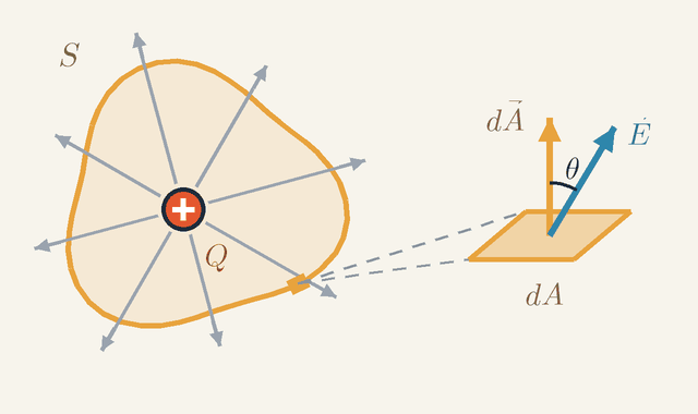
Figure 3. A closed surface S around Q, with one small patch enlarged: its area dA, its outward vector dA, and the field E at angle θ to it. The patch adds EdAcosθ to the flux.Legend
S
Closed surface around the charge; its shape can be anything.
Q
Charge inside S: the Qenc of Gauss's law.
C
dA
Area of one small patch of S.
m2
dA
The patch as a vector: length dA, pointing out of S at right angles to the patch.
m2
E
Field of Q at the patch.
N/C
θ
Angle between E and dA.
rad
Figure 3 shows a closed surface S around the charge Q, with one small patch drawn enlarged. The patch has area dA. To record which way it faces, make it a vector dA: of length dA, pointing out of S at right angles to the patch. The flux through the patch, the amount of field crossing it, is dΦ=E⋅dA=EdAcosθ where θ is the angle between the field E and dA. Only the part of the field that goes through the patch counts. A patch facing the charge squarely (θ=0) catches the most lines; tilted by θ, it catches fewer, by the factor cosθ; a patch the field only grazes (θ=90∘) catches none.
Adding the flux of every patch of S gives Gauss's law: ∮E⋅dA=ε0Qenc Here Qenc is the total charge enclosed by S, and ε0≈8.85×10⁻¹²F/m is the permittivity of free space, related to the Coulomb constant by k=1/(4πε0).
Why does the shape of S not matter? A solid angle is to a sphere what an angle is to a circle, and the whole sphere around a point is 4π. Seen from Q, the patch at distance r covers the small solid angle dΩ=dAcosθ/r2: its area as seen face-on from Q, divided by r2. Its flux is therefore EdAcosθ=r2kQdAcosθ=kQdΩ The r2 in the patch's apparent size cancels the 1/r2 of the field, so a small near patch and a large far one that cover the same solid angle carry the same flux.
The solid angles of a closed surface around Q add up to 4π, so the total flux is 4πkQ=Q/ε0, however bumpy S is. A charge outside S sends each of its lines in through one patch and out through another, giving as much negative flux as positive. That is why only the enclosed charge counts.
For the animation's +1 nC charge, the flux through any closed surface around it is 10−9/(8.85×10−12)≈113Vm. A surface around both charges has zero net flux: every line that leaves through it comes back in.
Two consequences follow. Shrinking the surface around a single point turns Gauss's law into a statement about that point, ∇⋅E=ρ/ε0: field lines begin and end only where there is charge. And with symmetry, Gauss's law gives fields with almost no calculation. A uniformly charged sphere acts, outside itself, like a point charge at its centre. A large flat sheet carrying σ coulombs per square metre sends its field straight out on both sides; a flat box of face area A straddling the sheet then has flux 2EA and encloses σA, so E=σ/(2ε0) on each side.
Equipotentials and the V(x) graph
An equipotential is a surface on which V has the same value everywhere. Moving a charge along it takes no work, and the spacing between neighbouring ones measures the field. A map of equipotentials therefore carries the same information as the field lines, often in a form that is easier to read.
In the expert layer of the animation, the dashed purple curves are equipotentials at ±400, ±150 and ±50 V, and the straight dashed line midway between the charges is V=0. They cross every field line at right angles. The reason: −∇V points the way V falls fastest, and that is straight across a surface on which V does not change at all. The gold charge starts at 393 V, just outside the 400 V curve, which cuts the axis 19.7 mm from the + charge.
Close spacing means a strong field, because V changes by the same amount over a shorter distance. The +50 V curve cuts the axis 21.3 mm from the midline, where V=0, so the average field over that gap is 50/0.0213≈2.35kV/m. That is a little above the 2.22 kV/m at the midpoint itself, because the field grows towards the charge.
The V(x) graph shows the same along the axis through the charges. Its slope is −Ex, minus the component of the field along the axis: about −2.2 V per millimetre at the midpoint, and ten times steeper where the trip starts. Outside the pair, V(x) rises with x on both sides, so there Ex<0: left of the + charge the field points away from it, right of the − charge it points towards it, and both directions are to the left. The gold dot slides down the curve as its potential energy U=qV turns into kinetic energy K.
Laplace's equation: no resting place
No stable trap for a charge can be built from fixed charges. The reason is one property of a single equation for V alone, found by combining the two results above.
Put E=−∇V into ∇⋅E=ρ/ε0. This gives Poisson's equation, ∇2V=−ρ/ε0, and in empty space, where ρ=0, Laplace's equation, ∇2V=0. The Laplacian ∇2V measures how much the average of V over a small sphere around a point exceeds its value at the centre. In empty space it is zero, so V at every point equals its average over any small sphere around it.
A value equal to the average of its surroundings can be neither above all of them nor below all of them. So in empty space V has no maximum and no minimum, only saddles. A positive charge would need a minimum of V to rest in stable equilibrium, so no arrangement of fixed charges can hold a charge stably (Earnshaw's theorem). For example, midway between two equal positive charges E=0, but a positive test charge there is pushed back only along the axis; sideways, it is pushed out. Atoms owe their stability to something else: quantum mechanics.
Conductors and the capacitor field
In a conductor some charges are free to move. That single fact fixes the field inside and just outside every conductor, and it explains the uniform field of a capacitor.
Free charges move as long as any field acts on them, so they stop only when the field inside the metal is zero. A conductor at rest is therefore a single equipotential. Any closed surface drawn inside the metal has zero flux, so by Gauss's law it encloses no charge: any excess charge sits on the surface. Just outside, the field is perpendicular to the surface, since a component along it would set the surface charges moving. A small flat box straddling the surface has flux only through its outer face, which gives the field's size, E=σ/ε0, with σ the surface charge per square metre.
Two parallel plates carrying +σ and −σ each make the sheet field σ/(2ε0). Between the plates the two fields point the same way and add; outside they point opposite ways and cancel. The result is the uniform field of a capacitor, E=σ/ε0=ΔV/d for plates a distance d apart.
The dipole seen from far away
A dipole is a pair of equal and opposite charges, a common source in nature: many molecules are dipoles. Far from it the two potentials nearly cancel, and what is left obeys a simple law of its own.
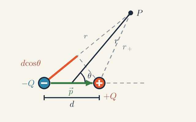
Figure 4. A dipole seen from a point P. When P is far away, the lines to it are nearly parallel and r− exceeds r+ by the segment dcosθ, which gives V≈kpcosθ/r2. Not to scale.Legend
Q
Size of each of the two charges, +Q and −Q.
C
d
Distance between the two charges.
m
p
Dipole moment: size p=Qd, pointing from −Q to +Q.
C⋅m
P
Point where the potential is found.
r
Distance from the centre of the dipole to P.
m
θ
Angle between p and the line from the centre to P.
rad
r+
Distance from +Q to P.
m
r−
Distance from −Q to P.
m
dcosθ
How much farther P is from −Q than from +Q, when P is far away: the part of d pointing towards P.
m
Figure 4 sets up the geometry. The charges +Q and −Q are a distance d apart. The dipole moment p has size p=Qd and points from −Q to +Q. The point P is at distance r from the centre of the pair, in a direction at angle θ from p, and at distances r+ and r− from the two charges. Adding the two point-charge potentials: V=kQ(r+1−r−1)=kQr+r−r−−r+
The result now depends on the small difference r−−r+. When P is far away compared with d, the lines from the two charges to P are nearly parallel. The dashed perpendicular from +Q meets the line from −Q to P; from that foot on, the remaining distance to P is almost exactly r+. So r− is longer than r+ by the thick segment from −Q to the foot, labelled dcosθ: the part of the separation d that points towards P. In the denominator the two distances hardly differ, so r+r−≈r2. Hence V≈r2kQdcosθ=r2kpcosθ
Because the two contributions nearly cancel, the potential falls as 1/r2 instead of 1/r, and the field, its gradient, falls as 1/r3. At a given distance, V is largest along p (θ=0), zero on the plane through the centre at right angles to p (θ=90∘), and negative on the side of the negative charge.
A check with the animation's pair: p=10−9⋅0.18=1.8×10⁻¹⁰Cm. At 1 m along the axis the formula gives 1.62 V, against the exact kQ(1/0.91−1/1.09)≈1.63V. The relative error is about d2/(4r2), here 0.8 %, so the approximation is already good at a distance of little more than five separations.
Worked problem: a proton and an electron
Energy conservation with the potentials found above gives speeds without solving any equation of motion. Comparing two particles then shows what depends on the mass and what does not.
Replace the gold charge by a proton, of charge e and mass mp, released from rest at the same point, 20 mm from the + charge. How fast is it at the midpoint, and at the end of the trip, 20 mm from the − charge? The potential falls by 393.3 V on the way to the midpoint, where V=0, and by 786.6 V on the way to the end. One electronvolt (eV), 1.602×10⁻¹⁹J, is the energy a charge e gains falling through one volt, so 21mpv12=e⋅393.3V=393eV,v1≈2.74×10⁵m/s 21mpv22=e⋅786.6V=787eV,v2≈3.88×10⁵m/s Twice the energy gives 2 times the speed.
Now release an electron, of charge −e and mass me, from rest at the far point. The force on it, −eE, points against the field, so it is pushed back towards the + charge, up the potential. The arrangement is symmetric, and the electron's potential energy −eV is the mirror image of the proton's, so it runs the same path in reverse and gains the same 787 eV, or 1.26×10⁻¹⁶J. Its mass is 1836 times smaller, so its speed is 1836≈42.8 times larger: 1.66×10⁷m/s, 5.5 % of the speed of light.
The size of any relativistic correction is set by the kinetic energy compared with the rest energy, K/(mec2)=787/511000≈0.15%, and it lowers that speed by only about 0.1 %.
Energy gives speeds, not times. For times we need the equation of motion along the axis, mx¨=qE(x). Divided by m, it depends on the particle only through q/m. So every particle with a charge of the same sign, released from rest at the same point, follows the same path, and if q/m is larger by some factor, the whole motion runs faster by its square root: all times scale as m/q.
The animation's charge is given a mass of about 49 mg so that its trip takes 4.0 s. The proton's q/m is 4.7×10¹³ times larger, so it makes the trip in 4.0s/4.7×1013≈0.58μs. The electron, 42.8 times quicker again, takes 13.6 ns.
Limits of validity
Every result above rests on assumptions. Knowing where they fail tells you when a larger theory is needed.
Sources at rest. Electrostatics assumes the charges stay put. News of a change at one charge reaches the other only after the light travel time, 0.6 ns across the animation's 180 mm, so the instantaneous Coulomb sum works only for charges that move slowly compared with light. When magnetic fields change, Faraday's law gives ∮E⋅dl=0: the work round a loop is no longer zero, and the field is no longer a pure gradient. It becomes E=−∇V−∂A/∂t, with A the magnetic vector potential.
Point charges. The inverse-square law is among the best-tested laws in physics: the exponent equals 2 to within about 10−15. The point charge, though, is an idealisation: its field energy, 21ε0E2 per cubic metre, adds up to infinity near a true point. At very short range quantum effects appear. Below about 4×10⁻¹³m, the reduced Compton wavelength of the electron, a probe passes inside the cloud of quantum vacuum fluctuations that partly screens every charge. It then sees more of the charge, so the force grows slightly faster than 1/r2, and this measurably shifts hydrogen's energy levels. Inside the hydrogen atom the field is about 5×10¹¹V/m; the electron there must be treated by quantum mechanics, though still in the Coulomb potential.
Matter and strong fields. In a material the field of a free charge is reduced by the relative permittivity, about 80 for water. Insulators also have limits: dry air breaks down and sparks at about 3 MV/m, and even empty space would start creating electron–positron pairs near 1.3×10¹⁸V/m.
Where this leads
In Capacitors, E=σ/ε0 and the energy 21ε0E2 per cubic metre describe the field between the plates. Electric Current and Resistance and DC Circuits and Ohm's Law follow charges driven through matter by a potential difference. Magnetic Force on Moving Charges adds qv×B to qE, and Special Relativity shows that the two fields are parts of one: what one observer calls a pure electric field, another sees as partly magnetic. Electromagnetic Induction breaks ∮E⋅dl=0, and Electromagnetic Waves shows the fields travelling on their own at c=1/ε0μ0. The same 1/r potential describes gravity in Gravitation and Orbits and holds the electron in Atomic Models: the Bohr Atom, where hydrogen's binding energy is 13.6 eV.
Key formulas
Electric field from the force on a test charge
E=qF
The field at a point is the force on a small positive test charge placed there, divided by that charge. Doubling the charge doubles the force, so the ratio describes the point, not the probe. A negative charge in the same field is pushed the opposite way, since F=qE with q<0.
Symbols
E
size of the electric field
V/m
F
size of the force on the test charge
N
q
test charge
C
When it holds: The test charge must be small enough not to move or disturb the source charges. On a moving charge a magnetic field adds its own force, qv×B.
Example: At the animation's midpoint the 0.1 nC charge feels 0.22 µN: E=2.22×10⁻⁷/10−10≈2.2×103V/m.
Field of a point charge
E=r2kQ
Coulomb's law divided by the test charge. The field points radially away from a positive charge and towards a negative one, and it falls as the inverse square of the distance, because the same number of field lines spreads over spheres of area 4πr2.
Symbols
E
size of the field
V/m
k
Coulomb constant, 8.99×10⁹
Nm2/C2
Q
source charge (its size, for the magnitude)
C
r
distance from the charge
m
When it holds: For a point charge, or outside a spherically symmetric charge, at rest in vacuum. For several charges, add the fields as vectors.
Example: The animation's +1 nC charge at the starting point, 20 mm away: E=8.99×109⋅10−9/0.0202≈2.25×104V/m.
Potential of a point charge
V=rkQ
The work per unit charge needed to bring a test charge from very far away, where V=0, to the distance r: the integral of kQ/r2 from r out to infinity. It falls as 1/r, not 1/r2, and keeps the sign of Q, so the potentials of several charges add as signed numbers.
Symbols
V
potential at the distance r, zero far away
V
k
Coulomb constant
Nm2/C2
Q
source charge, with its sign
C
r
distance from the charge
m
When it holds: For a point charge, or outside a spherical one, at rest in vacuum, with the zero of potential at infinity.
Example: At the animation's start, 20 mm from +1 nC and 160 mm from −1 nC: V=449.5−56.2≈393V.
Potential energy and the work of the field
ΔU=qΔV=−Wfield
Moving a charge q through a potential difference ΔV changes its potential energy by qΔV, and the field's own work is the negative of that. A positive charge moving to lower potential loses potential energy while the field does positive work and speeds it up; for a negative charge every sign flips.
Symbols
ΔU
change of electric potential energy
J
q
charge that is moved, with its sign
C
ΔV
potential difference, final minus initial
V
Wfield
work done on the charge by the electric field
J
When it holds: For electrostatic fields, where the work does not depend on the path. Fields induced by changing magnetic fields have no single-valued potential.
Example: The animation's 0.1 nC charge goes from +393 V to −393 V: ΔU=10−10⋅(−786.6)≈−78.7nJ, so the field does 78.7 nJ of work on it.
Field as the slope of the potential
E=−dxdV(E=−∇V)
The field component along any direction is minus the rate at which the potential changes along it. So the field points downhill in V, towards lower potential, is strongest where V changes fastest, and is perpendicular to the equipotentials. The gradient ∇V collects the three slopes into one vector.
Symbols
E
component of the field along x
V/m
V
electric potential
V
x
position along the chosen direction
m
E
electric field vector
V/m
∇V
gradient of the potential, pointing where V rises fastest
V/m
When it holds: For static fields. When magnetic fields change, E=−∇V−∂A/∂t.
Example: At the animation's midpoint V(x) falls by about 2.2 V per millimetre, so Ex≈+2.2kV/m, pointing towards the − charge.
Potential difference as a line integral
ΔV=−∫E⋅dl
Add up E⋅dl along a path from one point to the other and change the sign. Moving along the field lowers the potential, moving against it raises it, and moving across it changes nothing. This is the inverse of the gradient formula.
Symbols
ΔV
potential at the end minus potential at the start
V
E
electric field along the path
V/m
dl
small step along the path
m
When it holds: In electrostatics the result is the same for every path between the two points. With changing magnetic fields it depends on the path.
Example: Moving 1.0 cm along a uniform field of 50 kV/m: ΔV=−5.0×104⋅0.010=−500V.
Uniform field between parallel plates
E=dΔV(uniform field)
In a uniform field the line integral is just the field times the distance, so the field is the voltage divided by the gap. It points from the plate at higher potential to the one at lower potential, and its unit, the volt per metre, comes straight from this formula.
Symbols
E
size of the uniform field
V/m
ΔV
voltage between the plates
V
d
distance between the plates, measured along the field
m
When it holds: For plates much wider than the gap, away from their edges, where the field fringes outward.
Example: 500 V across plates 1.0 cm apart: E=500/0.010=5.0×104V/m, far below the 3 MV/m at which air breaks down.
Gauss's law
∮E⋅dA=ε0Qenc
The flux of the field out of a closed surface, the sum of E⋅dA over it, equals the charge enclosed divided by ε0, whatever the shape of the surface. It follows from the inverse-square law: for a point charge, E⋅4πr2=Q/ε0 at every radius. Charges outside the surface send in as many lines as they take out.
Symbols
E
electric field on the surface
V/m
dA
small piece of the surface, pointing outward
m2
Qenc
net charge inside the surface
C
ε0
vacuum permittivity, 8.85×10⁻¹²
C2/(Nm2)
When it holds: Holds for any closed surface, even for moving charges, but gives the field directly only when symmetry fixes its direction and size on the surface. In matter, the induced charges must be counted too.
Example: Any closed surface around the animation's +1 nC charge: flux =10−9/(8.85×10−12)≈113Vm; around both charges, zero.
Glossary
Electric field
The condition of space around charges that pushes on any charge placed there, F=qE. It exists whether or not a charge is there to feel it, and it has a size and a direction at every point.
Test charge
A small positive charge used to probe a field, too small to disturb the charges that produce it. The field is the force on it divided by its charge, so the result does not depend on how big it is.
Superposition principle for charges
Each charge produces its field as if the others were absent: fields add as vectors, potentials as signed numbers. Together with Coulomb's law it fixes every electrostatic field.
Electric field line
A curve that runs along the field at every point. Lines start on positive charges, end on negative ones, never cross and crowd where the field is strong; they are not, in general, the paths that released charges follow.
Electric potential
The potential energy per unit charge at a point, V=U/q, measured from a chosen zero, usually far away. A positive charge is pushed towards lower potential, a negative one towards higher potential.
Potential difference (voltage)
The difference of potential between two points: the work per coulomb done against the field in carrying a charge from one to the other. A 9 V battery gives 9 J to every coulomb it pushes round a circuit.
Equipotential surface
A surface on which the potential has the same value everywhere. Field lines cross it at right angles and moving a charge along it takes no work; the surface of a conductor at rest is one.
Conservative field
A field whose work on a charge moving between two points does not depend on the path, so that ∮E⋅dl=0 around any loop. Every electrostatic field is conservative, which is why a potential exists.
Electron-volt
The energy an electron gains when accelerated through 1 V, 1eV=1.602×10⁻¹⁹J. Atomic energies are a few eV; a proton accelerated through 100 V gains 100 eV.
Electric dipole
Two equal and opposite charges a distance d apart, like the pair in the animation. Far away their fields almost cancel: the potential falls as 1/r2 and the field as 1/r3.
Gauss's law
The flux of E out of any closed surface equals the charge inside divided by ε0, whatever the shape of the surface. For 1 nC the flux is about 113 V·m; it is the inverse-square law in geometric form.
Earnshaw's theorem
No arrangement of fixed charges can hold a charge in stable equilibrium in empty space, because the potential there has no minimum, only saddle points. Stable atoms need quantum mechanics.
Quantities
E
Electric field
V/m
The force per unit charge on a small positive test charge, a vector at every point; E is its size. 1 V/m is the same as 1 N/C.
q
Test charge
C
The charge that feels the field, F=qE; in the animation q=+0.1nC.
Q
Source charge
C
A charge that produces the field, positive or negative; the animation's are ±1nC.
r
Distance from the charge
m
The distance from a source charge to the point where the field or the potential is wanted.
k
Coulomb constant
N⋅m2/C2
The constant of Coulomb's law, k=1/(4πε0)≈8.99×109N⋅m2/C2.
ε0
Vacuum permittivity
C2/(N⋅m2)
The constant that sets how much field a charge produces in vacuum, 8.85×10⁻¹²C2/(N⋅m2); it appears in Gauss's law.
V
Electric potential
V
Potential energy per unit charge at a point, a signed number; 1V=1J/C. At the animation's start it is about 393 V.
ΔV
Potential difference
V
Final minus initial potential: the voltage between two points, which fixes the energy a charge gains or loses between them.
U
Electric potential energy
J
The energy of a charge due to its position in the field, U=qV; for the animation's test charge it falls from 39.3 nJ to −39.3 nJ.
F
Electric force
N
The force on a charge in the field, F=qE; 0.22 µN on the animation's test charge at the midpoint, 2.28 µN at the start.
Quiz
Beginner What does the arrow on an electric field line show?
The path every charge must follow
The direction an electron would be pushed
The direction a small positive charge would be pushed
Where the charge is stored
Show answer
Answer: C. The direction a small positive charge would be pushed
By definition, field lines show the push on a small positive test charge. An electron would be pushed the opposite way.
Beginner On a field-line map, where is the electric field strongest?
Where the lines are closest together
Where the lines are farthest apart
Where the lines are straight
It is the same everywhere
Show answer
Answer: A. Where the lines are closest together
The density of field lines shows the strength of the field: crowded lines mean a strong field.
Beginner The electric field at a point points to the right. A small negative charge is placed there. Which way is it pushed?
To the right
To the left
Upwards
It is not pushed at all
Show answer
Answer: B. To the left
Negative charges are pushed opposite to the field direction, so it is pushed to the left.
Intermediate A 2 nC charge placed at a point feels a force of 6 µN. What is the electric field there?
1.2 × 10⁻¹⁴ N/C
333 N/C
3 × 10⁻³ N/C
3000 N/C
Show answer
Answer: D. 3000 N/C
E = F / q = 6 × 10⁻⁶ ÷ (2 × 10⁻⁹) = 3000 N/C (= 3 kV/m). Multiplying instead of dividing gives 1.2 × 10⁻¹⁴.
Intermediate What is the field 10 cm from a point charge of 4 nC? (k = 8.99 × 10⁹ N·m²/C²)
360 V/m
3600 V/m
36 V/m
36 000 V/m
Show answer
Answer: B. 3600 V/m
E = k·Q / r² = 8.99 × 10⁹ × 4 × 10⁻⁹ ÷ 0.1² ≈ 3600 V/m. Forgetting to square r gives 360 V/m.
Intermediate A proton is accelerated from rest through a potential difference of 100 V. How much kinetic energy does it gain?
100 eV
100 J
1.6 × 10⁻¹⁹ eV
50 eV
Show answer
Answer: A. 100 eV
ΔK = q·ΔV = e × 100 V = 100 eV (about 1.6 × 10⁻¹⁷ J). The electron-volt is defined to make this simple.
Advanced Along the x-axis the potential is V(x) = 200·x² (V in volts, x in metres). What is E_x at x = 0.5 m?
+200 V/m
−50 V/m
−200 V/m
+50 V/m
Show answer
Answer: C. −200 V/m
E_x = −dV/dx = −400·x = −200 V/m. The minus sign means the field points towards decreasing x, downhill in V.
Advanced Two equal charges +Q are a distance d apart. With V = 0 far away, what are E and V at the midpoint?
E = 0 and V = 0
E = 0 and V = 4k·Q/d
E = 8k·Q/d² and V = 0
E = 8k·Q/d² and V = 4k·Q/d
Show answer
Answer: B. E = 0 and V = 4k·Q/d
The two fields are equal and opposite, so E = 0. Potentials are scalars and add: 2 × k·Q/(d/2) = 4k·Q/d. E = −∇V vanishes because V is stationary there (a saddle point), not because V is zero. For +Q and −Q it is the reverse: V = 0 but E = 8k·Q/d².
 Physics Tutor